Deep Determinsitic Policy Gradient Algorithm
Reinforcement Learning is good if it can be applied to practical siutations. A practical state may not always have a discrete set of action space. Imagine a self driving car learning to drive. There are numerous possibilities for the agent (i.e. self driving car). It can go left, speed up, accelerate etc… Degree of such motions may also change. Speed can go up to 98.5mph or 65.5mph. It is evident that action space is too large here, and discretizing it will bring up the curse of dimensionality.
Value based algorithms such as Q-learning, DQN, DDQN are all discrete action space algorithms. Poliy gradient algorithms such as REINFORCE, A2C, A3C can be modified to work for continuous actions as well. But these algorithms face challenges while interacting with higher dimensions.
All these shortcomings led to the evolution of Deep Deterministic Policy Gradient (or better known as DDPG) algorithm. In this article, we will talk about the evolution of DDPG both from the mathematical aspect as well as technical implementation side of things. So, warm up your coffee again, as we are doing deep here!
Need for DDPG?
Introduced in 2016, by Google Deepmind (again), DDPG has changed the course for RL and its research. But, why was it needed in the first place?
Most real-life tasks are continuous state - continuous action tasks. Hence, value based algorithms are not quite useful there. Besides, other PG algorithms are On Policy algorithms, i.e. improving only the policy that they are learning. That’s where the need of a newer algorithm comes. DDPG connects all the dots.
- It supports continuous state continuous action spaces
- It is an off policy algorithm, i.e. it can find the best policy even by learning from some other policy.
- Besides, it uses the best of the worlds of Value based and Policy Gradient algorithms
| Algorithm | Model | Episodic | Policy | Action Space | State Space | Learner |
|---|---|---|---|---|---|---|
Q-learning | Model free | No | Off-policy | Discrete | Discrete | Q-value |
SARSA | Model free | No | On-policy | Discrete | Continuous | Q-value |
DQN/DDQN | Model free | No | Off-policy | Discrete | Continuous | Q-value |
REINFORCE | Model free | Yes | On-policy | Discrete | Continuous | Policy \(\pi\) |
A2C/A3C | Model free | No | On-policy | Continuous | Continuous | Policy \(\pi\) |
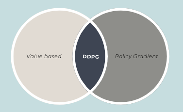
So, what is DDPG?
There are quite a few moving pieces in DDPG algorithm. I will try to explain the individual parts first, before connecting all of them together into the final algorithm. As mentioned earlier, DDPG gets the best of both value methods and PG methods. It utilizes concepts from DQN (a value method) while also learning the policy using PG method. So, let’s look at the individual pieces that are required for DDPG.
Moving Part 1: Deterministic Part
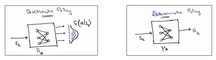
Let’s quickly recap on Policy Gradient methods such as REINFORCE or Actor Critic methods. All such methods talk about stochastic policy generation. The key idea of stochasticity is given a state, the agent gives you a probability distribution from which you can sample an action. Hence, the stochasticity.
Deterministic Policy, on the other hand, gives you the exact action which needs to be taken. Hence, the deterministic attribute.
Let’s hold on to the deterministic piece for a while.
Moving Part 2: Critic (from Actor Critic methods) combined with DQN
State value functions, or better termed as Q-value functions is represented as below:
\(Q^{\pi}(s_t, a_t) = \mathbb{E}[r(s_t, a_t) + \gamma.\mathbb{E}[Q^{\pi}(s_{t+1}, a_{t+1})]]\)
Note that above Bellman Equation has 2 expectations. What are these?
- The interior \(\mathbb{E}\) : as there are possibilities of many actions under stochastic policy \(\pi\), expectation is needed to get an average next Q value.
- The exterior \(\mathbb{E}\) : considering many possibilities of next states \(s_{t+1}\), again an expectation is needed.
What if we change the policy to a deterministic policy in above Bellman equation instead? Something like :
\(Q^{\mu}(s_t, a_t) = \mathbb{E}[r(s_t, a_t) + \gamma.[Q^{\mu}(s_{t+1}, a_{t+1})]]\)
Look that the interior \(\mathbb{E}\) is gone. Why? Since, we know that there is only 1 action that needs to be taken given a state (using the deterministic nature here)
There are certain nuances in the above equation. Since, \(Q^{\mu}\) only depends on the expectation of the environment, i.e. state transition probability, it is possible to learn \(Q^{\mu}\) using different behavior policy \(\beta\). Hence Q-learning using a deterministic policy is an off policy.
So, this is our critic. . Given a particular state \(s_t\) and taken an action \(a_t\), it evaluates the Q-value of that state-action pair. The concept is quite similar to a DQN network.
Moving Part 3: The Actor
Now, the actor here is supposed to come up with a policy. Note that it needs to be a deterministic policy. Hence, the actor network should have only 1 output, i.e. the action to be taken.
Similar to Actor Critic methods, we would like to maximize the performance of our agent given a state, i.e. \(max J(\theta^{\mu})\).
The \(\theta^{\mu}\) that maximizes the performance can be found using gradient ascent method. \(\theta_{t+1} = \theta_{t} + \alpha.\mathbb{E}[\nabla_\theta{J(\theta)}]\)
As shown in the paper by Silver et al(2014), 
A lot of math here. Let’s speak some English now! It would be better to do a side comparison of an Advantage based Actor vs DDPG Actor
| Attribute | Advantage Actor | DDPG |
|---|---|---|
Policy Gradient | \(\nabla_\theta{J}(\theta) \propto \mathbb{E_\pi}[{A_t}.\nabla_\theta{log}\pi_\theta(s/a)]\) | \(\nabla_{\theta^\mu}{J} \propto \mathbb{E}[\nabla_a.Q(s,a :\theta^{Q}).\nabla_{\theta_\mu}\mu(s:\theta^\mu))]\) |
Update parameter | proportional to Advantage value | if critic value increases by changing action, means change in action is good for policy. That’s \(\nabla_a.Q(s,a)\) |
Moving Part 4: Encourage Exploration
- In DQN, exploration was performed using some action exploration techniques such as \(\epsilon\)-greedy.
- In PG method, since it generates a stochastic policy, exploration is inherent.
So, how can we have exploration in DDPG?
As highlighted in Lillicrap et al, the exploration can be treated independently of the learning algorithms. A new exploration policy \(\mu{'}\) is constructed by adding noise sampled from a noisy process N. ![]()
Moving Part 5: Updating the networks
Since the network \(Q(s, a|\theta^Q)\) being updated is also used in calculating the target value, the Q update is prone to divergence.
The solution to this is similar to target networks used in DQN. A copy of both actor and critic networks is created, so called target networks. These target networks are updated as below, taken from Lillicrap et al: 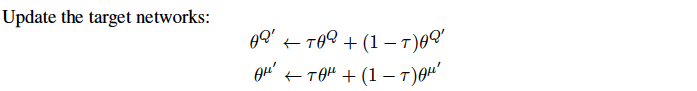
Unlike DQN, where the learnt network is copied onto the target network completely; here, target network is slowly updated, which greatly improves the stability of learning. Here, \(\tau << 1\).
Phew! So many new concepts introduced for DDPG. Let’s try to connect them together to form a Deep Deterministic Policy Gradient Algorithm (DDPG).
The Algorithm
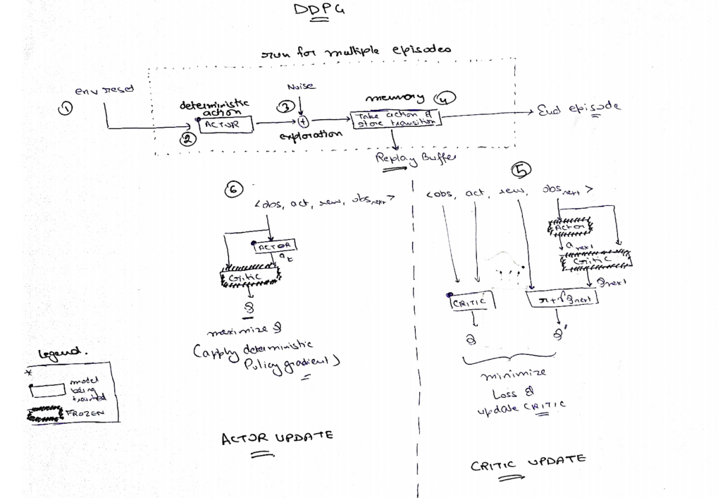
Let’s connect all the moving pieces together now.
Deepmind paper provides a psuedo code for DDPG algorithm, which is relatiely intuitive to comprehend. 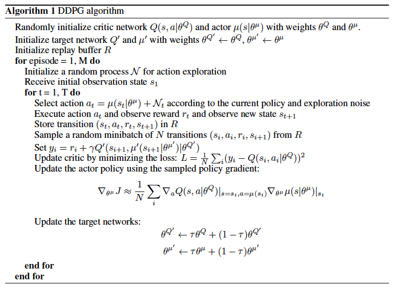
I have taken a step further, and tried to make a flow diagram for this algo.
Now, lets move on the implementation part of it.
The Implementation
With keras as my choice of Neural network framework, I will explain the step by step implementation of the DDPG algorithm.
Again, for detailed and full code, please reach out to me directly.
Memory Buffer
Similar to a DQN network, we will create a separate class for replay buffer, which can handle updates and sampling.
  class ReplayBuffer():
      def __init__(self, bufferSize, input_shape, n_actions):
          self.bufferSize = bufferSize
          self.memCounter = 0

          # create storage for state, action, reward and next states
          print((self.bufferSize, *input_shape))
          self.mem_state = np.zeros((self.bufferSize, *input_shape))
          self.mem_action = np.zeros((self.bufferSize, n_actions))
          self.mem_nextstate = np.zeros((self.bufferSize, *input_shape))
          self.mem_reward = np.zeros(self.bufferSize)         # reward is a scalar quantity
          self.mem_terminal = np.zeros(self.bufferSize, dtype=np.bool)

      def update(self, state, action, reward, nextState, dead):
          index = self.memCounter % self.bufferSize

          self.mem_state[index] = state
          self.mem_action[index] = action
          self.mem_reward[index] = reward
          self.mem_nextstate[index] = nextState
          self.mem_terminal[index] = dead

          self.memCounter += 1

      def sample(self, batchSize):
          if self.memCounter >= batchSize:

              # uniformly sample from the memory
              availableSamples = min(self.memCounter, self.bufferSize)

              sampleIndices = np.random.choice(availableSamples, batchSize, replace = False)

              states = self.mem_state[sampleIndices]
              actions = self.mem_action[sampleIndices]
              rewards = self.mem_reward[sampleIndices]
              nextStates = self.mem_nextstate[sampleIndices]
              terminals = self.mem_terminal[sampleIndices]

              return states, actions, rewards, nextStates, terminals

          else:
              return None, None, None, None, None
Actor Network
Implementing the actor network is straight forward. We will use keras Model subclassing Key point to note here is that actor network only returns 1 single action, since it is a deterministic action. Also, the activation function used for the last layer is a tanh function which range counds the action value from -1 to 1.
  class ActorNetwork(keras.Model):
      # keras model submoduling
      def __init__(self, action_size, name = "Actor", chkpt_dir = "/models/ddpg"):

          super().__init__()
          self.model_name = name
          self.n_actions = action_size            # only 1 action to be outputted, but this represents the size of action vector
          self.chkpt_dir = chkpt_dir
          if not os.path.exists(self.chkpt_dir):
              os.makedirs(self.chkpt_dir)

          self.layer1 = Dense(units = 400, activation="relu")
          self.layer2 = Dense(units = 300, activation="relu")

          # Also, as per the paper, the last layer had weights initialized
          last_init   = tf.random_uniform_initializer(minval = -0.003, maxval = 0.003)
          self.mu     = Dense(units = self.n_actions, activation="tanh", kernel_initializer=last_init)


      def call(self, state):
          prob = self.layer1(state)               # 1st layer returns a probabiltiy (since relu unit)
          prob = self.layer2(prob)              # 2nd layer returns a probabiltiy (since relu unit)
          action = self.mu(prob)                  # get the action using last layer

          return action
Critic Network
2 separate networks are used for Actor and Critic. Critic network follows a similar implementation as actor network. Only major difference is that Critic network is a Q-value function. Hence, it needs state and action as inputs.
  class CriticNetwork(keras.Model) :
      def __init__(self, name = "Critic", chkpt_dir = "\models\ddpg"):
          super().__init__()
          self.model_name = name
          self.chkpt_dir = chkpt_dir

          if not os.path.exists(self.chkpt_dir):
              os.makedirs(self.chkpt_dir)

          self.layer1 = Dense(units = 400, activation="relu")
          self.layer2 = Dense(units = 300, activation="relu")
          self.Q      = Dense(units = 1, activation="linear")

      def call(self, state, action):
          actionValue = self.layer1(tf.concat([state, action], axis = 1))         # input is a combination of state and action
          actionValue = self.layer2(actionValue)
          actionValue = self.Q(actionValue)
          return actionValue
The Agent
As always, we will implement the agent in its own class. While initialization, we will need to have 4 separate networks. 1 set is for Actor-Critic networks. The other set is the target Actor-Critic networks, which are softly updated as the agent learns.
Although DDPG paper talks about OU process for noise generation. In our implementation, we use gaussian noise for simplification.class DDPG(): def __init__(self, env, dim_state, n_actions, discount_factor = 0.99, tau = 0.005, batch_size =64, noise = 0.1, \ bufferSize = 1000000, save_dir = None, **kwargs): self.discount_factor = discount_factor self.tau = tau # represents the soft target update rate self.batch_size = batch_size self.n_actions = n_actions self.max_action = env.action_space.high[0] self.min_action = env.action_space.low[0] # create the memory self.ReplayBuffer = buffer.ReplayBuffer(bufferSize=bufferSize, input_shape=dim_state, n_actions=n_actions) # create the noise process self.noise = noise # create the networks self.save_dir = f"{pref}/models/Policy/DDPG" if save_dir is None else save_dir self.Actor = networks.ActorNetwork(action_size=n_actions, chkpt_dir=self.save_dir) self.Critic = networks.CriticNetwork(chkpt_dir = self.save_dir) self.targetActor = networks.ActorNetwork(action_size=n_actions, chkpt_dir=self.save_dir, name = "TargetActor") self.targetCritic = networks.CriticNetwork(chkpt_dir = self.save_dir, name = "TargetCritic") # compile the networks learning_rate_actor = kwargs["learning_rate_actor"] if "learning_rate_actor" in kwargs.keys() else 0.0001 learning_rate_critic = kwargs["learning_rate_critic"] if "learning_rate_critic" in kwargs.keys() else 0.001 self.Actor.compile(optimizer = optimizers.Adam(learning_rate=learning_rate_actor)) self.Critic.compile(optimizer = optimizers.Adam(learning_rate=learning_rate_critic)) self.targetActor.compile(optimizer = optimizers.Adam(learning_rate=learning_rate_actor)) self.targetCritic.compile(optimizer = optimizers.Adam(learning_rate=learning_rate_critic)) # update the target network with main networks self.updateNetworks(tau = 1)Target Networks need to be updated with every training. Here is a quick implementation where we update both actor & critic target networks.
  def updateNetworks(self, tau = None):
      # updates the target networks
      tau  = self.tau if tau is None else tau
      # tau is required for the soft update of the network weights as described in the paper

      # Actor update
      weights = []
      for index, weight in enumerate(self.Actor.weights):
          _thisweight = tau*weight + (1-tau)*self.targetActor.weights[index]
          weights.append(_thisweight)
      self.targetActor.set_weights(weights)

      # Critic Update
      weights = []
      for index, weight in enumerate(self.Critic.weights):
          _thisweight = tau*weight + (1-tau)*self.targetCritic.weights[index]
          weights.append(_thisweight)
      self.targetCritic.set_weights(weights)
Action Selection while also exploring the environment is imminent here. As explained above, we add a noise to the action chosen by our deterministic actor for exploration. Now, one thing that we need to ensure is that after adding the noise, action may go beyond the range defined. Hence, we will clip the action to make it range bound again.
  def getAction(self, state, mode = "TRAIN"):
      # given the state, get the action.
      # exploration needed if model is in training model
      state = tf.convert_to_tensor([state], dtype = tf.float32)
      action = self.Actor(state)
      if mode.upper() == "TRAIN":
          action += tf.random.normal(shape=[self.n_actions], mean=0.0, stddev=self.noise)
      action = tf.clip_by_value(action, self.min_action, self.max_action)
      return action
Replay buffer update is a simple update function as in DQN
  def updateMemory(self, state, action, reward, nextState, terminal):
      self.ReplayBuffer.update(state, action, reward, nextState, terminal)
Training the Agent: Now, this is the most important and rather complex part of all. We will use custom loss functions, both for critic and actor & train them appropriately.
Critic Loss is represented as: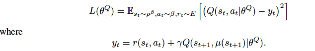
In case of actor, we simply want to maximize the Q-value generated from Critic network. The deterministic policy gradient is presented as: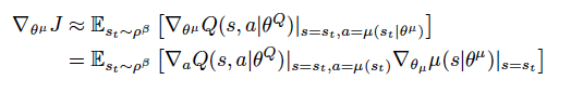
  def train(self):
      # this is the heart of DDPG
      if self.ReplayBuffer.memCounter < self.batch_size:
          return
      # sample a batch from memory
      states, actions, rewards, nextStates, terminals = self.ReplayBuffer.sample(self.batch_size)

      states = tf.convert_to_tensor(states, dtype = tf.float32)
      actions = tf.convert_to_tensor(actions, dtype = tf.float32)
      rewards = tf.convert_to_tensor(rewards, dtype = tf.float32)
      nextStates = tf.convert_to_tensor(nextStates, dtype = tf.float32)
      terminals = tf.convert_to_tensor(terminals, dtype = tf.bool)

      # Critic Update
      with tf.GradientTape() as tape:
          actions_next = self.targetActor(nextStates)
          q_next = self.targetCritic(nextStates, actions_next)
          target_q = rewards + self.discount_factor*q_next

          # critic generated q
          current_q = self.Critic(states, actions)
          # loss
          loss_critic = losses.MSE(target_q, current_q)

      grad_critic = tape.gradient(loss_critic, self.Critic.trainable_variables)
      self.Critic.optimizer.apply_gradients(zip(grad_critic, self.Critic.trainable_variables))

      # Actor Update
      with tf.GradientTape() as tape:
          actions_actor = self.Actor(states)
          q_values = self.targetCritic(states, actions_actor)
          # aim is to maximize q_values --> minimize -qValues
          loss_actor = -q_values

      grad_actor = tape.gradient(loss_actor, self.Actor.trainable_variables)
      self.Actor.optimizer.apply_gradients(zip(grad_actor, self.Actor.trainable_variables))

      # now update the network parameters with soft update
      self.updateNetworks(tau = self.tau)
Run the whole scene
With all the knobs in place, let run the agent with the below set of code.
  actor_params    = {"learning_rate_actor": 0.0001}
  critic_params   = {"learning_rate_critic": 0.001}
  save_dir        = f"/models/Policy/DDPG"
  env             = gym.make('Pendulum-v0')
  nbEpisodes      = 250
  Agent           = DDPG( env, dim_state = env.observation_space.shape, n_actions =  env.action_space.shape[0],  \
                      discount_factor = 0.99, tau = 0.005, batch_size =64, noise = 0.1, bufferSize = 1000000, save_dir = save_dir, **actor_params, **critic_params)

  mode = "TRAIN"
  for _thisepisode in tqdm(range(nbEpisodes)):
      _currentState = env.reset()
      _episodicReward = 0
      _dead = False
      while not _dead:
          action = Agent.getAction(_currentState, mode = mode)

          # perform the action
          _nextState, _reward, _dead, _info = env.step(action)
          _nextState = np.squeeze(_nextState)
          _reward = np.squeeze(_reward)

          Agent.updateMemory(_currentState, action, _reward, _nextState, _dead)
          Agent.train()

          # update States
          _currentState = _nextState
          _episodicReward += _reward

          # if game over, then exit the loop
          if _dead == True:
              logger.info(f'Episode: {_thisepisode+1} Steps: {_thisstepsTaken} Reward:{_episodicReward} ')
              break
Conclusion
Again, DDPG was a lot to digest. But, atleast, we learnt quite a lot here. DDPG has changed the direction of reinforcement learning. So, it becomes critical to understand the ins and outs of DDPG.
A quick peak of the overall learning through above implementation. 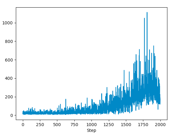
As the master agent progresses, the episodic reward reached new highs. The running average of the reward also goes up! 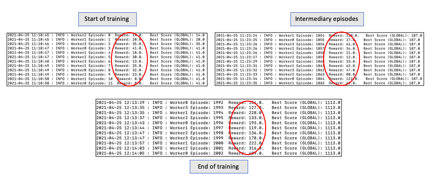
With this, we come to an end of DDPG and its explanation. Pour another coffee now to stay kicking!
Appendix
References
- DPG Paper by Silver et al. Deterministic Policy Gradient Algorithms
- DDPG Paper by Lillicrap et al. Continuous Learning with Deep Reinforcement Learning
- Sunny Guha Medium Article
- Olivier Sigaud Youtube Lecture
- Phil Tabor Youtube Lecture