Policy Gradient - REINFORCE
In this article, we will talk about the foundation Policy Gradient algorithm: REINFORCE.
The underlying idea here is to reinforce actions which result in higher cumulative rewards. In simple words, the algorithm increases the probability of action if it results in more rewards.
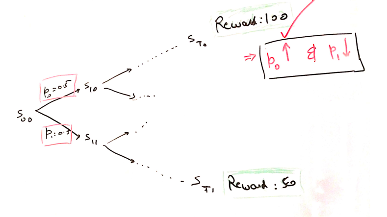
As in below figure,
- \(a_0\) with probability(\(p_0\)): 0.5 results in cumulative reward of 100.
- \(a_1\) with probability(\(p_1\)): 0.5 results in cumulative reward of 50.
Hence, increasing \(p_0\) will result in higher rewards on average.
REINFORCE works on this simple idea. Ofcourse, the internal mathematics and technicalities are more complex than above diagram.
Digging Deeper - Mathematically
We would like to learn a policy that can take best actions without consulting the value functions. It becomes a conventional optimization problem as below:
Objective: \({max} {J}(\theta)\), where \({J} {, } \theta\) refer to performance measure and policy parameters respectively.
Using stochastic gradient ascent, we update \(\theta\) in the direction of \(\nabla_\theta{J(\theta)}\).
\(\theta_{t+1} = \theta_{t} + \alpha.\mathbb{E}[\nabla_\theta{J(\theta)}]\)
It turns out that computing gradient of performance is further simplified to:
\(\nabla_\theta{J}(\theta) \propto \mathbb{E_\pi}[{G_t}.\nabla_\theta{log}\pi_\theta(s/a)]\)
where \(G_t\) is the discounted return
Hence, \(\theta\) udpate is re-written as : \(\theta_{t+1} = \theta_{t} + \alpha.G_t.\nabla_\theta{log}\pi_\theta(s/a)\)
Key takeaways from above equation:
- \(\nabla_\theta{J}\) is independent of states distribution.
- \(\theta\) is updated in proportion to return. If higher return is achieved by taking a particular action, then the probability of taking that action rises in proportion.
Quick peek into the Algo
Before we delve into the detailed algorithm, here are few tacts related to REINFORCE:
- A Monte Carlo based method, i.e. it needs knowledge of full episode before learning.
- An On Policy algorithm, i.e. only learns the policy which decides the actions.
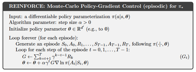
Here is a snippet of psuedo code taken from Sutton and Barto’s RL Book
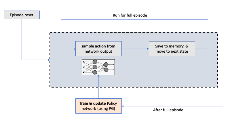
A rough REINFORCE flow looks like:
Implementation
There are many implementations available on the web, and I will not write another one here. The idea wanted to highlight is certain nuances while implementing this algorithm. So, sip your coffee slowly now!
- Policy Network:
- Input – state vector
- Method 1: Update the target values in policy network
- Predicted Value – Network’s predicted log probabilities (since softmax is the output layer)
- Target Value –
- Since, the probability of a promising action should be strengthened, we can use an updated target value
- \(\pi(s/a) : \pi(s/a) + \beta.\nabla_\theta{J}\), which further reduces to
- \(\pi(s/a) : \pi(s/a) + \beta.G.\nabla_\theta{log}\pi_\theta(s/a)\).
- Loss function – Cross entropy.
- Cross Entropy Loss : \(L = \sum(y_i.{log p_i})\)
Our Policy Gradient also seeks for log of probability
  # p_i --> action probability
  # y_i --> 1 for chosen action and 0 for not chosen action
  # beta --> learning rate for policy network
  # G --> discounted Rewards

  gradient = -(p_i - y_i)           # this is the gradient of cross entropy loss

  # update the target value by gradient
  y_target = p_i +  beta * G * gradient
- Method 2: Update policy network parameter \(\theta\) directly using tensorflow eager execution
- Custom Loss Function –
  losses = []         # accumulate losses

  # start eager execution
  with tf.GradientTape() as tape:
      for index, sample in enumerate(self.memory):
          # sample is a tuple of current state, actions, rewards, next states

          # get current state in the memory variable
          state = tf.Variable([sample[0]], trainable=True, dtype=tf.float64)

          # given current state, get prob of actions using policy network
          prob = self.PolicyNetwork.model(state, training = True)

          # actual action taken, and taking the log of probability of actual action taken
          action = sample[1]
          actionProb = prob[0, action]
          logProb = tf.math.log(actionProb)

          # loss of this sample is defined as G*log(p) --> this is as per policy gradient
          sampleloss = logProb * discounted_rewards[index][0]

          losses.append(-sampleloss)      # this is negative, since we are interested in gradient ascent


      networkLoss = sum(losses)

      # Back propagation
      # compute the gradient of network loss wrt network parameters, and optimize the network
      grads = tape.gradient(networkLoss, self.PolicyNetwork.model.trainable_variables)
      self.PolicyNetwork.optimizer.apply_gradients(zip(grads, self.PolicyNetwork.model.trainable_variables))
- Custom Loss Function –
- Training the agent:
- Since this is Monte carlo method, agent can only learn once the entire episode has ended
NOTE: Please reach out to me directly for detailed code
Challenges & Potential Solutions
Being a basic algorithm, REINFORCE is bound to have certain challenges of its own.
High Variance and slow learning
Problem
- With cumulative rewards varying a lot every episode, the overall lerning becomes a bit noisy with high variance.
- A better way to reduce the noise is to normalize the rewards used. This is what we have now
\(\theta_{t+1} = \theta_{t} + \alpha.G_t.\nabla_\theta{log}\pi_\theta(s/a)\)
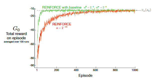
Solution
- Reinforce with Baseline – > If we amend the reward by a function which is independent of action taken, the overall learning becomes faster.
\(\theta_{t+1} = \theta_{t} + \alpha.(G_t - b(s_t)).\nabla_\theta{log}\pi_\theta(s/a)\)- How do we choose baseline:
- Normalize Cumulative rewards: \(G_t - b(s_t) = (G_t - \mu(G_t))/\sigma(G_t))\)
- Use Value function as baseline. \(G_t - b(s_t) = G_t - V(s_t)\)
Episodic Learning
Problem
- Being a Monte carlo method, knowledge of entire episode is required.
- Becomes impractical in more real-life scenarios when you dont know what may happen in the environment
Solution
- We need to move towards Temporal Difference (TD) methods; which we will learn more about in next articles
Conclusion
Here, we learnt about the most basic Policy Gradient alogrithm. Ofcourse, this is just to do some warm up while we work out further deep into PG techniques.
Appendix
References
- Reinforcement Learning, An Introduction (Second Edition). Sutton and Barto
- Karpathy Github page
- Lilianweng Github Page