Actor Critic Methods
Policy Gradient are “cool” algorithms to make the agent learn. We saw how REINFORCE, as simple as it is, can help learn the agent. With few tricks, such as baseline methods, learning variances can be reduced further. Next in line of the Policy Gradient techniques is Actor Critic (AC) Methods. First introduced in 2013 through the paper Natural Actor-Critic Algorithms, they now set a foundation to a series of advanced AC methods (A2C, A3C), which we will dig further in later articles.
So, lets begin with the need of AC methods in the first place before we jump onto the mathematical technicalities.
A case for Actor Critic methods?
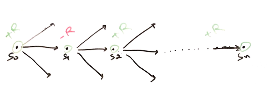
Dont need Full episode – A fully Monte Carlo method, REINFORCE needed a complete knowledge of entire episode before the policy could learn. In above episode, \(a_1\) taken at \(s_0\) turns out to generate negative reward. So, why run entire episode to discredit action \(a_1\)?
Actor Critic methods comes handy in this case, as they use Temporal Difference (TD) learnings.Critic to judge the performance – Imagine you (actor) are learning to ride a bike. You paddle hard! But your mom (critic) tells you to paddle harder! That’s what Actor Critic is. Another agent to evaluate the performance under current policy. Simple, isnt it?
Actor Critic
Quick recap of the Policy gradient (REINFORCE) equation:
\(\nabla_\theta{J}(\theta) \propto \mathbb{E_\pi}[{G_t}.\nabla_\theta{log}\pi_\theta(s/a)]\) , where \(G\) is defined as expected rewards if started from state \(s\)
Adding a baseline leaves us at:
\(\nabla_\theta{J}(\theta) \propto \mathbb{E_\pi}[({G_t - b_t(s))}.\nabla_\theta{log}\pi_\theta(s/a)]\) ,
But here is the catch. Both the formulations require a full episodic knowledge! Actor Critic Methods are one step ahead in a way that they utilize TD methods to perform online learning .
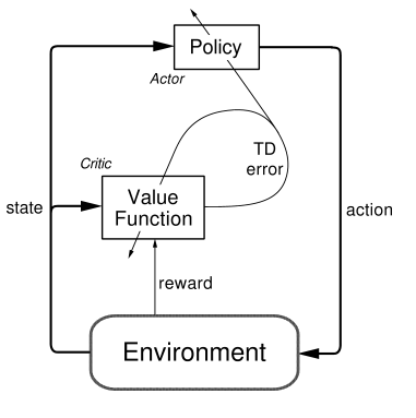
The policy network acts as an actor, whereas a value network acts as a critic which evaluates how good or bad the updated policy is at every step.
Here is a visualization of the architecture used in AC method. A lot to digest here. So, sit back and relax while I try to brew the math here :)
Value Function:
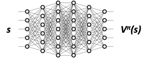
Given a state under a policy \(\pi\), this function approximator returns the value of that state, i.e. \(V_\phi^\pi(s)\).
How do we create this function approximator? This, in essence, is similar to Q-learning methods. Here is a quick summary:
Training data: \({ (s_{i, t}, y_{i, t} = r(s_{i, t}, a_{i, t}) + \gamma.V_\phi^\pi(s_{t+1}))}\)
Loss function (supervised regression): \(L(\phi) = 1/2(\sum_i ( V_\phi^\pi(s_{t}) - y_i)^2)\)
In the above training data, we just need only next step value, instead of entire episode. Loss function is simply defined as the Mean squared TD(1) error.
Using a simple NN can help achieve the above function.
Policy Network:
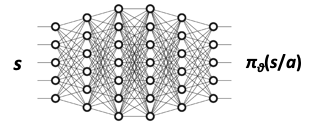
The policy network works as usual (similar to REINFORCE), with a slight change. Instead of using the entire episodic discounted reward to update \(\theta\), we will use the below update methodology, wherein we have the TD error (or Advantage ):
\(\theta_{t+1} = \theta_{t} + \alpha.A_t^\pi.\nabla_\theta{log}\pi_\theta(s/a)\), where
\(A_t^\pi\) is the TD error, mathematically formulated as: \(r(s_{i, t}, a_{i, t}) + \gamma.V_\phi^\pi(s_{t+1}) - V_\phi^\pi(s_{t})\)
Training data: \({ (s_i, y_i = \pi_\theta(s_t/ a_t) + \beta.A_t.\nabla_\theta{log}\pi_\theta(s/a))}\).
Loss function (cross entropy): \(L(\theta) = \sum_i(-y_i.{log(\pi_\theta)})\)
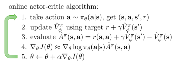
Sneak peak into the Algorithm
Implementation
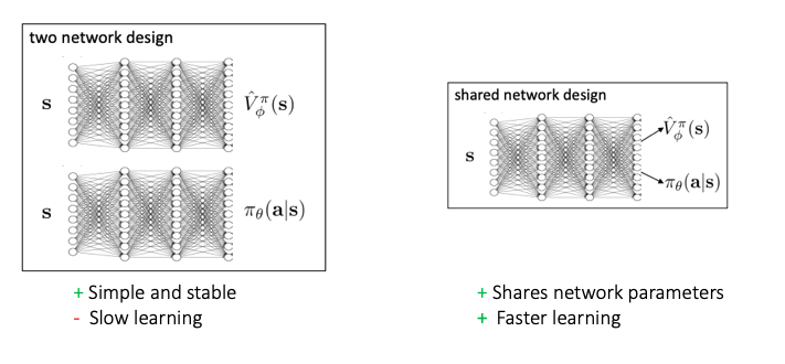
1. Network Design (2 vs 1)
Since, there are 2 separate learnings happening in AC methods, at first glance, it makes sense to use 2 separate networks to learn the policy and value functions separately. But, there is another school of thought which lets us use a dual network design as below:
2. Batch vs Online Learning
Online learning will require the parameter update at every step. Although technically feasible, but an update after every step makes the network unstable. Hence, all the updates wil happen after the end of each episode, i.e. batch learning in this case.
3. Actor & Critic learning
Since, we have a dual shared network, we can combine the losses as below:
\(L = L_{actor} + L_{critic}\)
- Actor Loss
\(L(\theta) = \sum_i(-y_i.{log(\pi_\theta)})\) Critic Loss
\(L(\phi) = 1/2(\sum_i ( V_\phi^\pi(s_{t}) - y_i)^2)\)
or, we can replace it with huber loss to make it differential everywhere.with tf.GradientTape() as tape: # sample --> tuple of current state, actions, rewards, next states, value (given current state) # get log prob state = tf.Variable([sample[0]], trainable = True, dtype=tf.float32) nextState = tf.Variable([sample[3]], trainable = True, dtype=tf.float32) action, reward, dead = sample[1], sample[2], sample[4] # run shared network to get action prob distro and value associated with that state actionProbDistro, _currStateValue = self.SharedNetwork(state, training = True) _actionProbDistro, _nextStateValue = self.SharedNetwork(nextState, training = True) # compute TD error # delta = r + gamma*V_(t+1) - V_t delta = reward + self.discountfactor* tf.squeeze(_nextStateValue) * (1 - int(dead)) - tf.squeeze(_currStateValue) # compute critic loss loss_sample_critic = delta**2 # compute actor loss actionProb = actionProbDistro.numpy()[0, action] loss_sample_actor = tf.math.log(actionProb) * delta networkLoss = loss_sample_critic + loss_sample_actor # performing Backpropagation to update the network grads = tape.gradient(networkLoss, self.SharedNetwork.trainable_variables) self.SharedNetwork.optimizer.apply_gradients(\ (grad, var) for (grad, var) in zip(grads, self.SharedNetwork.trainable_variables) \ if grad is not None)NOTE: Please reach out to me directly for detailed code
Conclusion
While REINFORCE was just an actor based method, we see that if we add a critique to criticise the policy learning, we can achieve a stable performance over time. Next in the article series are A2C and A3C, which are further developments in the actor-critic worlds.
Supplementary Read (for enthusiast learners)
So far, we only talked about TD based critic. But, you can ask whether that’s the only way to criticise the policy? The answer, ofcourse, is NO. Listed below are some other known critics that are available in literature.
- Q Actor-Critic
- Advantage Actor-Critic
- TD Actor-Critic
- TD(λ) Actor-Critic
- Natural Actor-Critic
Appendix
References
- Reinforcement Learning, An Introduction (Second Edition). Sutton and Barto
- University of California, Berkeley - Youtube Lecture
- University of California, Berkeley - Lecture slides
- Lilianweng Github Page
- Phil Tabor’s Youtube Page