Asynchronous Advantage Actor Critic Methods
The name Asynchronous Advantage Actor Critic Methods is quite a mouthful. From now on, we shall call it, just like it is called in academica world, A3C method. Introduced by Google Deepmind, again, in 2016, A3C methods have significantly picked up pace. Its simplicity, robustness and speed in standard RL tasks has made policy gradients and DQN obsolete.
In this article, we will dig deeper into A3C algorithm both from mathematical persective as well as implementation angle.
A3C - an understanding.
Let’s break down the 3As of A3C methods:
Asynchronous:
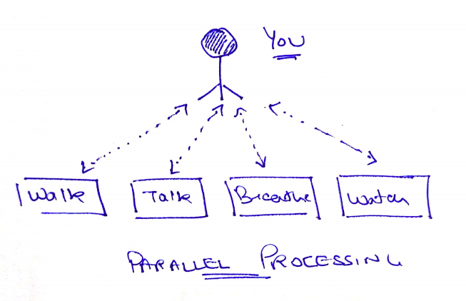
In computer engineering, parallel processing and asynchronization acts as a backbone. Here is a quick snap explaining parallel processing more intuitively.
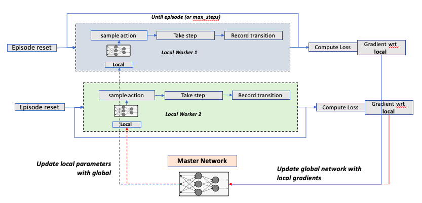
So, how is this concept used here? The below image (taken from: A Brandom-ian view of Reinforcement Learning towards strong-AI) summarizes the asynchronous concept in A3C methods quite elegantly.
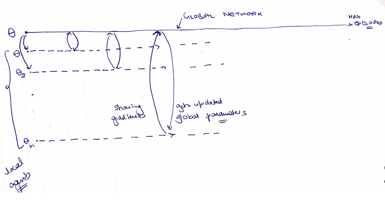
At the top of it, there is a master Network, which maintains a global set of parameters. Learning in parallel are local worker agents with their own set of Actor Critic models and parameters. Parameters are shared between global and local networks asynchronously as shown in the second image below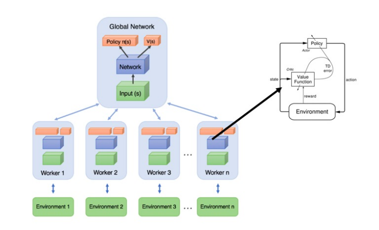
Okay. Parallel Processing is a “cool” concept. But why here? What do we get from asynchronous learning?
- Efficient Memory management. In DQN, we used an experience replay buffer to store state transitions. For more real situations, the memory requirements could go to million transitions (or more. Ofcourse, more is better). But was that efficient? No! Using asynchronous learning, we are achieving similar goal of recording state transitions through multiple agents.
- Faster Learning. Well, more agents are now learning the best policy now in parallel. If ought to have faster training time.
Advantage:
Advantage is a mere metric which tells the advantage of taking a particular action. Mathematically, k step advantage is written as \(A(s_t, a_t; \theta, \theta_v) = \sum_i \gamma^i.r_{t} + \gamma^k.V(s_{t+k, \theta_v}) - V(s_t, \theta_v)\)
In actor critic method article, we learnt about how advantage functions can be used efficiently to make actor critic learning more stable.Actor:
As simple as it may sound now, actor is simply the policy network, i.e, it learns the probability distribution of actions given a particular state \(\pi(a_t| s_t, \theta)\)
Critic:
Critic is simple the value function which criticizes how good or bad the policy is. You can dig deeper into it in the previous article.
The Algorithm
Deepmind paper provides a psuedo code for A3C algorithm, which is relatiely intuitive to comprehend. 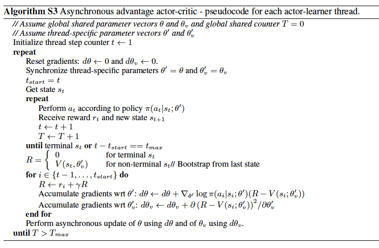
I have taken a step further, and tried to make a flow diagram for this algo. In the flowchart, I have added 2 local agents which learn in parallel while getting the latest parameters from the master network.
Now, lets move on the implementation part of it.
The Implementation
As always, I will use keras as my choice of Neural network framework with tensorflow as backend. The idea for this implementation came from this wonderfully explained tensorflow blog
Actor Critic Model
This is a common model utilizing keras Model subclassing .
Here, I will have 2 separate networks for actor and critic.class ActorCritic(keras.Model): def __init__(self, state_size, action_size): super().__init__() self.state_size = state_size self.action_size = action_size # create 2 separate models for actor and critic # --- Actor --> returns prob distribution for all possible states given state self.dense1 = Dense(units = 128, activation= "relu") self.policy = Dense(units = self.action_size, activation="softmax") # --- Critic --> Value function (given a state) self.dense2 = Dense(units = 128, activation= "relu") self.values = Dense(units = 1, activation="linear") def call(self, inputs): # forward pass hidden_policy = self.dense1(inputs) probs = self.policy(hidden_policy) hidden_value = self.dense2(inputs) values = self.values(hidden_value) return probs, valuesMemory Management
We need to store state transitions for every episode. At the end of the episode, we will reset this storage. Hence, the memory requirements are not as extensive as DQN networks. We will use simple lists to store required values.
  class Memory():

      def __init__(self):
          self.reset()

      def reset(self):
          self.states = []
          self.rewards = []
          self.actions = []

      def update(self, state, action, reward):
          self.states.append(state)
          self.rewards.append(reward)
          self.actions.append(action)
Master Agent
MasterAgent Class will have 2 key ideas:
- Global Model: This is set as an Actor Critic model that we had created earlier
- Shared Optimizer: Deepmind paper talks about different optimizers in the paper, but shared optimizer had the best performance of all. The shared optimizer takes the gradients from different workers, and updates the global parameters accordingly.
  class MasterAgent():
      def __init__(self, game, save_dir, **kwargs):
          self.Name = "A3C"
          self.gameName = game
          self.save_dir = save_dir
          if not os.path.exists(self.save_dir):
              os.makedirs(self.save_dir)

          # create the master environment
          env = gym.make(self.gameName)
          self.state_size = env.observation_space.shape[0]
          self.action_size = env.action_space.n

          # create a shared optimizer. Note the use of use_locking
          self.optimizer = tf.compat.v1.train.AdamOptimizer(learning_rate=kwargs["learning_rate"], use_locking=True)

          # setup a global network
          self.globalModel = Models.ActorCritic(state_size=self.state_size, action_size=self.action_size)

          # construct the global Model with some random initial state
          self.globalModel(tf.convert_to_tensor(np.random.random((1, self.state_size)), dtype = tf.float32))
This master network needs to be trained with paraellely running local agents.
  def train(self):
      # This is where multiple local agents are defined
      # Different agents are run & trained on dfferent threads.
      reward_queue = Queue()      # a queue to record episodic rewards across all agents
      cores = multiprocessing.cpu_count()
      print(f'Created {cores} threads')

      # global counter
      global_episode_index = multiprocessing.Value("i", 0)

      # create individual processes
      processes = []
      for _thread in range(cores):
          # create each agent object
          worker = WorkerAgent(state_size = self.state_size, action_size = self.action_size, \
                  global_model = self.globalModel, sharedOptimizer = self.optimizer, \
                  result_queue = reward_queue, global_episode_index = global_episode_index, \
                  workerIndex = _thread, gameName = self.gameName , save_dir = self.save_dir)

          p = threading.Thread(target = worker.run)
          p.start()
          processes.append(p)

      # wait for all worker agents to complete
      [p.join() for p in processes]

      # some code to show final summary of all rewards
Local Worker Agent
Local workers are individual Actor critic networks in itself, with their own set & state of environment. We keep track of which global episode this local worker is currenly running on.
Agent Initialization: Important thing to note that Local worker class inherits from Threading class module, as it shares some parameters across different workers.
class WorkerAgent(threading.Thread): # inheriting multiprocesing properties from Threading class best_score = 0 def __init__(self, state_size, action_size, global_model, sharedOptimizer, \ result_queue, global_episode_index, workerIndex, gameName , save_dir): super().__init__() self.state_size = state_size self.action_size = action_size self.globalModel = global_model self.optimizer = sharedOptimizer self.result_queue = result_queue # global episode as worker start index self.worker_episode_index = global_episode_index # create the local model self.localModel = Models.ActorCritic(state_size=self.state_size, action_size=self.action_size) self.Name = f'Worker{workerIndex}' self.gameName = gameName self.env = gym.make(self.gameName).unwrapped # unwrapped to access the behind the scene dynamics of gym environment self.save_dir = save_dir- Agent Learning: Each worker works independently of other worker until maximum number of episodes are encountered. Each episode will run as usual, i.e. :
- Reset environment & memory
- Run the episode
- sample action from probability distribution out of local network
- take step with action
- store the transition
- if training_condition, perform training.
Important part is the training. The below code explains how the local network is trained.
- Network losses are computed using eager execution (tensorflow GradientTape). Details of losses are further below.
- Gradient of the losses are computed with respect to local network
- Global network is then optimized with these local gradients
- Local parameters are reset with global parameters
def run(self): # runs the Agent forever (until all games played) # trains the agent while sharing the network parameters memory = Memory() total_steps = 1 while self.worker_episode_index.value < MAX_EPISODES: # run the agent for each episode current_state = self.env.reset() memory.reset() episodic_reward = 0 episodic_steps= 0 self.episodicLoss = 0 done = False while not done: # play the episode until dead # sample the action based on prob distribution from local model probs, _ = self.localModel(tf.convert_to_tensor(current_state[None, :], dtype = tf.float32)) action = np.random.choice(self.action_size, p = probs.numpy()[0]) # since probs is a tensor. need to convert to array # take a step towards the action next_state, reward, done, _ = self.env.step(action) if done: reward = -1 episodic_reward += reward memory.update(current_state, action, reward) # store the transition in memory if total_steps%T_MAX == 0 or done: # --- this is where the local model is being trained and global model gets udpated # track the variables involved in loss computation using GradientTape (eager execution) with tf.GradientTape() as tape: total_loss = self.compute_loss(done, next_state, memory) self.episodicLoss += total_loss # compute the gradients with respect to local model grads = tape.gradient(total_loss, self.localModel.trainable_weights) # THIS IS IMPORTANT # push the local gradients to global model and udpate global network parameters # then, pull teh global weights to local model self.optimizer.apply_gradients(zip(grads, self.globalModel.trainable_weights)) self.localModel.set_weights(self.globalModel.get_weights()) memory.reset() total_steps += 1 current_state = next_state episodic_steps += 1 # we are not using it print(f'{self.Name} Episode: {self.worker_episode_index.value} Reward: {episodic_reward}. ') with self.worker_episode_index.get_lock(): # update the global episode numner self.result_queue.put(episodic_reward) self.worker_episode_index.value += 1 # once the agent has exhausted all runs self.result_queue.put(None) - Loss Computation: Deepmind paper talks about the losses in detail. Let’s break down the losses.
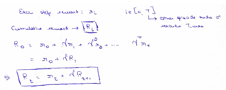
Discounted rewards computation We stored rewards generated after taking the actions. For advantage computation, we would need the discounted accumulated rewards. Let’s consider only 1 step returns for ease of explanation (rather than k step returns)
Feed Forward values Get probability distribution and state values by running the local network onto states present in memory
Advantage Computation Simply discounted reward - values
Critic Loss Defined as squared error \(L(\theta_v) = \sum_t(V_{\theta_v}^\pi(s_{t}) - A_t)^2\)
Actor Loss \(L(\theta) = \sum_t(-A_t.{log(\pi_\theta)})\)
Entropy Loss Defined explicity in the paper to avoid pre-mature convergence \(H(\theta) = \sum_t(-\beta.\pi_\theta.{log(\pi_\theta)}) , {where} \beta = 0.01\)
I had to go through some rough tricks of the trade to make it working. GradientTape eager execution is quite handy if you know how to use it properly. By default, all variables are watched by the tape. Also, all the variables need to be a tensor in order to be tracked by the tape. That’s the reason you will see a lot of convert_to_tensor in the below segment. Fail to do so will result in a non tensor variable, which is assumed to be a constant, and hence no gradient computation.
  def compute_loss(self, done, next_state, memory, discount_factor = 0.99, beta_entropy = 0.01):

      # get the reward value at final step
      if done:
          reward_sum = 0
      else:
          _, values = self.localModel(tf.convert_to_tensor(next_state[None, :], dtype=tf.float32))
          reward_sum = values.numpy()[0]

      # get discounted returns
      discounted_rewards = []
      for reward in memory.rewards[::-1]:
          reward_sum = reward + discount_factor*reward_sum
          discounted_rewards.append(reward_sum)

      discounted_rewards.reverse()
      discounted_rewards = np.array(discounted_rewards).reshape(-1,1)

      # forward run the netwrok to get probabilities and value functions for all states in memory
      probs, values = self.localModel(tf.convert_to_tensor(np.vstack(memory.states), dtype = tf.float32))

      advantages = discounted_rewards - values
      advantages = tf.convert_to_tensor(advantages, dtype = tf.float32)

      # critic loss
      loss_critic = tf.math.square(advantages)

      # actor loss
      # get probability of action taken
      actions= [[index, item] for index, item in enumerate(memory.actions)]
      prob_action = tf.convert_to_tensor(tf.gather_nd(probs, actions)[:, None])

      loss_actor = tf.math.log(prob_action + 1e-10)
      loss_actor *= - tf.stop_gradient(advantages)    # as per paper, advantages here is asusmed to be independent of parameter

      # entropy loss
      loss_entropy = tf.math.log(prob_action + 1e-10)
      loss_entropy *= - prob_action

      # total loss
      total_loss = tf.reduce_mean(loss_actor + beta_entropy*loss_entropy + loss_critic)
      return total_loss
The above implementation can be executed directly by following set of commands.
optimizer_args = {"learning_rate": 1e-4}
model = MasterAgent(game = "CartPole-v0", save_dir=save_dir, **optimizer_args)
model.train()
Conclusion
Phew, the whole A3C method was a lot, just like its name. But, overall it sets a new benchmark for performance in RL agents. As mentioned earlier, with faster execution, and more stable learning, A3Cs are preferred over other techniques.
A quick peak of the overall learning through above implementation. 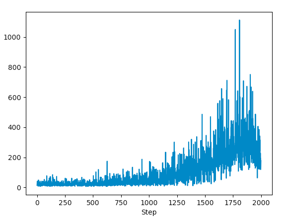
As the master agent progresses, the episodic reward reached new highs. The running average of the reward also goes up! 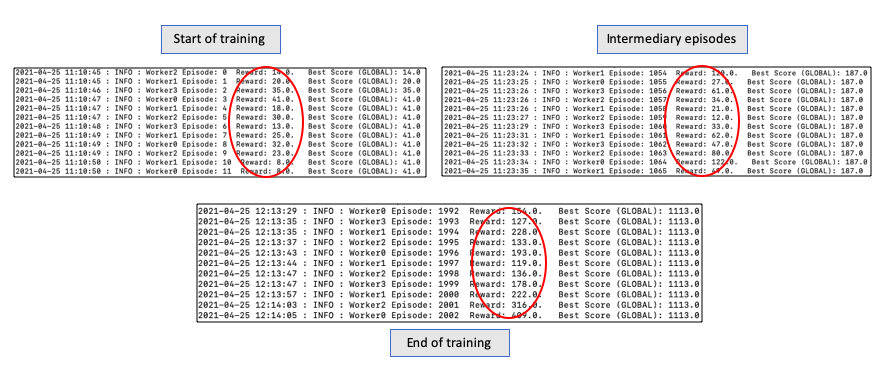
With this, we come to an end of A3C and its explanation. Pour another coffee now to stay kicking!
Appendix
References
- A3C Paper Asynchronous Methods for Deep Reinforcement Learning
- Tensorflow blog on A3C implementation- Blog
- Lilianweng Github Page
- AI Summer Page Actor Critic Methods
- Phil Tabor Youtube Lecture