Design your own Fractal
My last article in the Fractals series was devoted to the understanding of Fractals from the most basic perspective. Being extensively used in Computer graphics, this article will present a way to create and design your own fractals.
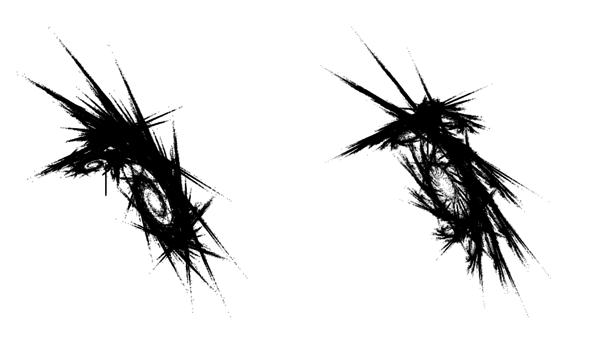
2 different fractal images are presented here. With a slight difference in the inputs, a whole new image is generated. Isn’t that fascinating! So, let’s make our hands dirty and get on board with the how of designing.
Iterated Functions System (IFS)
Before we design our first Fractal, we need to understand the self similarity attribute. In computer science and mathematics, an iterative (or even a recursive) function can achieve self similarity.
\(f({X_t}_1) = k * f(X_t) + c\), where \(\lvert k\rvert \lt 1\).
Such a recursive function when applied to graphics, generate a pattern like below
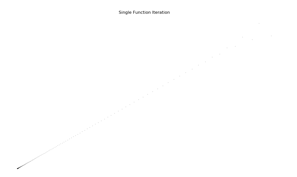
This is just a dotted line, with relative spacing increasing with number of iterations. Starting at point (0,0), the same linear transformation and translation is applied iteratively. This Transformation matrix is given by: \(\begin{bmatrix} .81 & .44 \\ .50 & -.48 \end{bmatrix}\) (generated randomly)
Note - If you want to brush up a little bit on Linear Algebra, I would recommend 3B1B youtube series
If recursively drawing a single function generates a brush paint pattern, now you can imagine what would it like be if we combine multiple transformations and draw them recursively. This idea is referred to as Iterated Functions System
Sierpinski Triangle
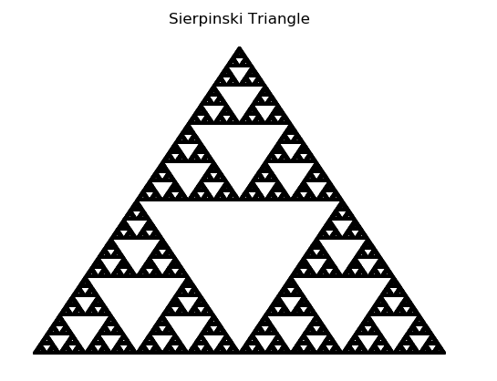
A very famous fractal image is also the most simplistic one. Lets break it down piece by piece
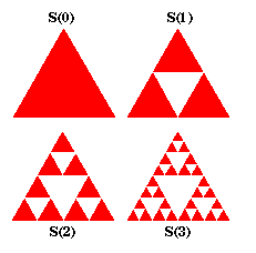
The Iterated Function System(IFS) for this image can be presented as:
- Begin with a starting object
- Reduce the object into half of the size and make 3 copies (3 function systems )
- Align them in the shape of an equilateral triangle. (represented by the translation vector)
- Go to step #2.
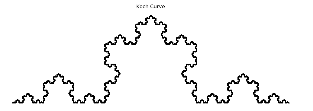
Koch Curve
Another great example is Koch Curve. Let’s look at the system of functions required to bring this fractal into life.
 \[f_1(x) = \begin{bmatrix} 1/3 & 0 \\ 0 & 1/3 \end{bmatrix}x \qquad f_2(x) = \begin{bmatrix} 1/6 & -\sqrt{3}/6 \\ \sqrt{3}/6 & 1/6 \end{bmatrix}x + \begin{bmatrix} 1/3 \\ 0 \end{bmatrix} \qquad f_3(x) = \begin{bmatrix} 1/6 & \sqrt{3}/6 \\ -\sqrt{3}/6 & 1/6 \end{bmatrix}x + \begin{bmatrix} 1/2 \\ \sqrt{3}/6 \end{bmatrix} \qquad f_4(x) = \begin{bmatrix} 1/3 & 0 \\ 0 & 1/3 \end{bmatrix}x + \begin{bmatrix} 2/3 \\ 0 \end{bmatrix}\]
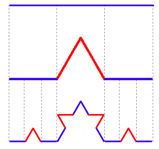
This system of equations represent the following iteration methodology:
- Begin with a starting object
- Reduce the object into 1/3 of the size and make 4 copies (4 function systems )
- Rotate 1 copy by 60°
- Rotate another copy by -60°.
- The last copy is just the replica of original object but 1/3 of size
- Repeat steps 2-5.
I hope these 2 examples must have given a brief flavour on how Fractals are generated. Applying certain Transformations repeatedly can lead to a whole other object altogether.
What’s next now?
This is just the beginning of what fractals are capable of. Art is just a way to visualise mathematics. Here, I present to you few more Fractal images. Try to guess the Transformations that could have led to these fractals.
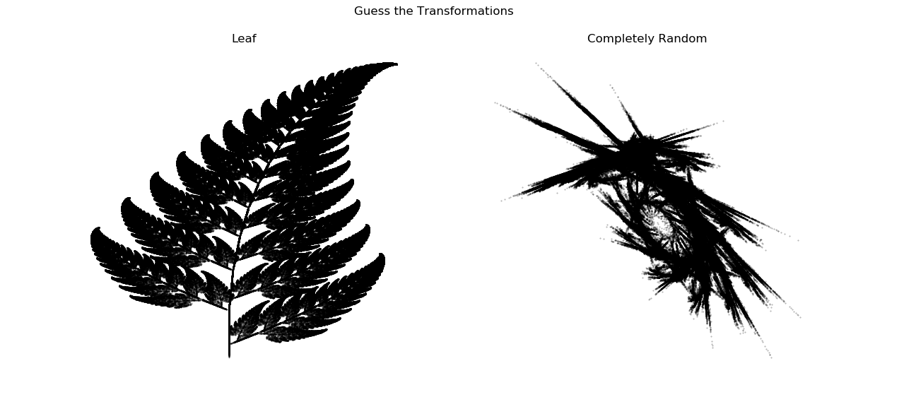
So far, we have only covered the Linear Transformations that can be applied to any object. Can there be more such transformations? Can we add a randomness to a randomness? Stay tuned for the next article to find out more.
Note - In case anyone is interested for the source code (written in Python) to generate these image, please contact me directly!