Order Execution using RL
Moving further in our series of Reinforcement Learning and its applications in Finance, this article talks about Order Execution in Financial Markets. A classic problem like this, laid the foundations of RL in Finance. One of the very early papers (Reinforcement Learning for Optimized Trade Execution by Yuriy Nevmyvaka et al) in 2005-06. The early penetration into RL gives an idea how important this problem is.
In this post, we will give a high level description of the problem statement before jumping onto the RL based solution. At the end, we will compare the results of different RL techniques alongside some base level market adopted (non RL) algorithms.
Problem Description
Traders (or market agents), everyday, face the challenge of executing a bulk order, i.e. Buy \(N\) shares of a particular asset. The goal is to purchase in such a manner so as to minimize the effective cost of purchase. A simple example is as below:
| Time | Available Inventory | Executed Size | Purchase Price |
|---|---|---|---|
10:00 | 10000 | 2000 | $125.3 |
10:15 | 8000 | 1000 | $126.4 |
10:30 | 7000 | 4000 | $122.1 |
10:45 | 3000 | 3000 | $123.0 |
In the above example, the initial order got executed in 45 minutes in different batches. The example is a made up scenario, ofcourse. Effectively, there should be a systematic way to get these orders executed in small batches so as to have a minimum impact cost.
GOAL: Hence, in the use case of Optimized Order Execution, our aim is to minimize the impact cost while also reduce (maximize) the effective buy (sell) price.
We will make this problem a continuous space - discrete action problem.
Data Requirements
- Asset Class: Stocks (RELIANCE, SAIL)
- Market: India
- Data Type: OHLCV (Open, High, Low, Close, Volume)
- Data Frequency: OHLCV level data available every minute.
- Data Period: Training 2018, 2019 Testing 2020
- Data Source: Sourced from here
NOTE: We have restricted our use case to OHLCV type of data. In such problems, Limit Order Book or Tick-By-Tick data could have proven to be more suitable. Researches by Yuriy et al have shown that LOB data is better here.
However, the cost of purchasing such data goes in thousands of dollars. If you have such data, we can explore improving the execution algorithms using TBT or LOB data.
Mathematical Formulation
The mathematical formulation is adapted from Almgren & Chriss, 2000 The agent has \(V\) of a security and wants to completely liquidate before time horizon \(T\). We divide \(T\) into \(N\) intervals of length \(\tau = T/N\) and specifically, discretised times \(t_k = k\tau\) for \(k = 0,1,…,N\).
Moreover, let a trading trajectory be the sequence \(q_0, …, q_N\) where \(q_k\) is the number of units we hold at time \(t_k\) or the inventory, and consequently \(x_k = q_k - q_{k-1}\) is the units of shares to be executed at time \(t_k\).
Alongside, we define that orders to be executed should always be a multiple of \(m { lotsize}\). Hence, \(x_k\) can take values from \(0, m, 2m, ...(V/m)m\).
Let’s summarize the parameters used here:
| Parameter | Summary | Value or Domain |
|---|---|---|
| \(V\) | Units to purchase (or liquidate) | 10000 |
| \(T\) | Time Horizon to purchase (liquidate) | 100 minutes |
| \(N\) | Orders to be executed in N individual intervals | 50 |
| \(\tau\) | Interval length \(T/N\) | 2 minutes |
| \(m\) | lot size, i.e. orders to be sent in multiples of m | 500 |
| \(x_k\) | lots executed at time \(t_k\) | ranges from \(1\) to \(V/m\) |
Our initial holding is \(q_0 = V\) and at \(T\), we require \(x_N = 0\)
The agent enters into the environment, and takes step, i.e. the order gets executed. There are certain assumptions made of the environment:
[1] A market order is sent,
[2] The order gets fully executed at Close Price at that time.
[3] Other market agents’ interaction with the market is not included.
[4] The order to be executed on same day before market close
Let’s define the attributes pertaining to this environment.
Actions
The actions are discretized for the use case. Since, the trading trajectory defines above highlights \(x_k\) as units executed at time \(t_k\). Hence, \(a_t \in [0,V/m]\) where \(a_t\): action to taken at time step \(t\).
     self.action_space = ActionManager.DiscreteActionSpace(actions = \
                     list(np.arange(int(self.initialOrderSize/ self.orderSizeFactor)+1)))
The code snippet is taken from my RL library. As always, for detailed code, please reach out to me directly
State
The state space defined for the use case is quite simplistic in nature. As mentioned above, due to lack of LOB data availability, we have limited the environment to utilize OHLCV data. Below are the attributes defining the state space
- Price Vector: Last \(n_{history}\) minutes Close price. Normalized to day’s open price. Length: \(n_{history}\)x1
- Volume Vector: Defines current traded volume as per OHLC V. Normalized by historical 1 minute traded volume. Length: 1x1
- Open Inventory: At the start of current state, # of units left to be executed. Normalized to initial open order. Length: 1x1
- Time left: Time left in the overall time horizon. Represented in % terms for normalization. Length: 1x1
Total length of state vector:
\(n_{history}.1 + 1 + 1 + 1\)This way of state creation is quite simplistic in nature, and ofcourse will not be able to model the Order Execution environment in complete sense. Hence, this kind of solution aims at Partially Observable Markov Decision Process (POMDP)
Reward
As in all RL problems, reward formulation is quite an art. Order Execution problem has been researched many times. It is one of the most sought after optimization problems in the fields of Finance. We will consider different reward methodologies here
- Vanilla Reward (VR): The below described method is quite simplistic in nature and here, immediate reward \({r_t}\) has 3 key components:
- Revenue from Executed Order: Executed order * change in Price from last time stamp.
- Order Impact Penalty: Penalty imposed for higher order size. Higher the order size, more the impact cost and higher penalty.
- Reward for taking additional step: Distributing order execution to multiple steps reduces order size, and hence reduces the chance on higher impact cost.
Hence, immediate action is given as below: \(r_t = \delta_{price}.x_t + \beta_{impact} * x^2_{t_N} + \beta_{timestep} * step\) - Almgren Chriss Reward (ACR): The reward and utility functions are described in Almgren & Chriss, 2000. I have not included this reward feature in this exercise, but will encourage reader to try this reward methodology.
- Vanilla Reward (VR): The below described method is quite simplistic in nature and here, immediate reward \({r_t}\) has 3 key components:
Terminal State
The agent will terminate when either of the below conditions are met:
- All inventory is executed before time horizon \(T\)
- Time horizon \(T\) reached. If this happens, all remaining inventory is executed immediately as a market order.
Objective
The agent’s objective is to maximize the discounted cumulative rewards:
\(max \mathbb{E}[\sum_t \gamma^t.r_t]\), where \(\gamma: {discount factor}\)
Summarizing generic parameters used in creating the environment
| Hyperparameter | Value | Description |
|---|---|---|
Asset Ticker | RELIANCE | Listed on NSE. One of the most liquid stocks in Indian market |
Inventory | 10000 | Initial inventory to liquidate (or purchase) |
Time Horizon | 100 mins | All inventory to get executed within this time frame |
Execution Start time | 9:30AM | NSE opens at 9:15 AM. Execution starts after 15 minutes |
nHistory | 15 mins | Number of historical records used in state vector |
Impact Penalize | -100 | Penalize factor for impact cost |
Step Reward | 0.1 | Reward for taking an extra step |
Reinforcement Learning Agents and Network Topologies
We will use couple of RL algorithms (agents) utilizing both the worlds of Value based methods and Policy gradient methods
Single layer DQN (DQN-SL) and 3 Layer DQL (DQL-3L)
For a detailed understanding of DQN, I would recommend the Deepmind paper in Nature. I will not go in the technicalities of DQN, but its application in this specific case.

Similar structure is used for 3 Layer DQN structure. Only difference being the number of Dense + Dropout layers
Network Configuration as below:
Hyperparameter Value Description mini batch size32 number of training cases over which each Adam Optimizer is run replay memory buffer10000 updates are sampled from this memory target network update frequency50 The frequency (measured in number of episodes) to update the target network optimizerAdam Adam optimizer is used to train the network learning rate0.001 Optimizer learning rate clip value100 Clips the final output of network to be between this -100 to 100 initial exploration1 initial value of \(\epsilon\) in \(\epsilon\) greedy exploration final exploration0.1 final value of \(\epsilon\) in \(\epsilon\) greedy exploration final exploration frame6000 number of frames over which \(\epsilon\) is linearly annealed to final value DDQN 3 Layer (DDQN-3L)
Similar to DQL-3L structure, Double DQN differs from DQN in the internal mechanics of how the target values are computed. Again, I will not go into the details of such difference, but will suggest this wonderfully written post here.
Network architecture is similar to DQN-3L.
Single Layer A3C (A3C-SL) and 3 Layers A3C (A3C-3L)
The details of A3C can be googled on internet, and I wont go into the technicalities and mathematics behind it. As a recommendation, please read this paper Asynchronous Methods for Deep Reinforcement Learning

Network Configurations (same for actor and critic) as below:
Hyperparameter Value Description mini batch size32 number of training cases over which each Adam Optimizer is run Number of cores4 Number of cores on which the worker agents are trained optimizerAdam Adam optimizer is used to train the network learning rate0.001 Optimizer learning rate Network Layers1 (3) Dense Layer of 20 neurons each for Actor and Critic
Loss functions utilized in individual DQN and A3C agents are similar to the ones used in respective papers (DQN, A3C) published.
Let’s compare the performance of these individual learning agents.
Agent Performance Evaluations
The entire exercise is solely developed in Python (3.8+). For NN networks, keras has been used with tensorflow as backend.
As always, for detailed code and explanation, please write to me directly.
Without further ado, lets jump onto the agents and their learning patterns. For all the agents, the training period was 2018 and 2019. Every time, the environment is reset, a day is sampled, and order execution happens on that sampled date.
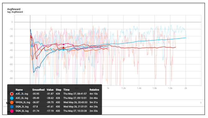
So, what’s happening here?
There are 5 different agents learning to work their way around the environment
- DQN-SL:
- Number of episodes: 1000 episodes
- Saturation stared happening after 1st 200 episodes
- DQL-3L:
- Number of episodes: 1000 episodes
- Saturation stared happening after 1st 400 episodes.
- A bit of slower learning than a single layer network. Extra layers dont add much value. Slows down the network due to vanishing gradients.
- DDQN-3L:
- Number of episodes: 1000 episodes
- Higher variance, and slower learning than DQN-SL.
- A3C-SL:
- Number of episodes: 2000 episodes
- Number of cores: 3 cores
- Similar performance to DQN-SL, but faster learning as running on multiple cores
- A3C-3L:
- Number of episodes: 2000 episodes
- Number of cores: 3 cores
- Best performance of all. Seems like even after 2000 episodes, agent was still learning. Reward saturation wasnt achieved yet.
The below graphical summary compares the number of steps taken to fully execute the order 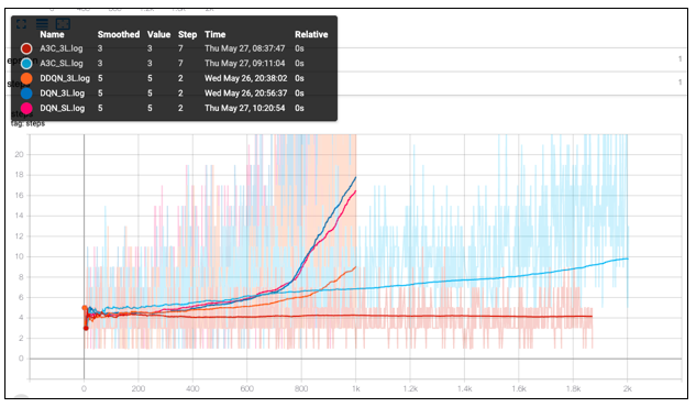
- DQN networks learnt to spread the inventory across multiple intervals. Number of steps taken start rising sharply.
- A3C networks are slow to learn in that aspect. A3C-3L started distributing the orders to multiple steps only after having gone through many episodes.
Agent Testing
In order to test the performance of our agent(s), we will compare them against a base case of Equally executed orders at equal time intervals.
Base Case:
- Inventory to purchase: 10000.
- Lot size: 500
- Time Horizon: 100 minutes with 50 intervals.
- Execution: 1 lot every 2 minutes for 20 intervals. This way, all the inventory will be executed.
Test Date: 31 JAN 2020
1. Stock: RELIANCE
Reliance is a fairly liquid stock in Indian markets. For more details on daily traded volume, please refer to NSE India)
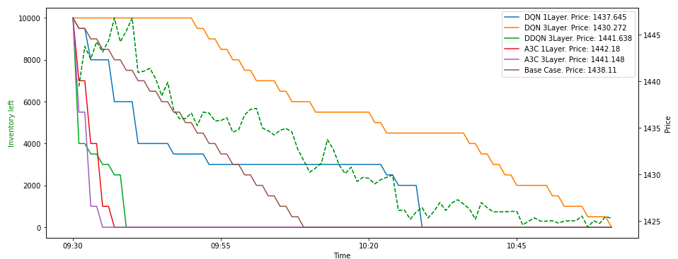
Key Takeaways:
- DQN-3L has given us the best executed price. Orders spread across till the last minute, the agent has tried to minimize the impact cost while also giving us the best execution price
- Both A3C agents sent out big orders and the entire inventory got executed immediately
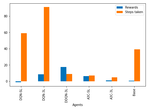
2. Stock: SAIL
Reason for choosing SAIL is because of its liquidity. It is not as heavily traded stock as Reliance, but has a relatively good volume. I will say it is a mid tier liquid stock.
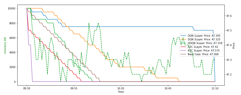
Key Takeaways:
- Price movement is very limited in case of Sail. In the time frame, it has moved between 47.1 to 47.8.
- Again, DQN agents show the best execution here. With higher reward, better execution price, and order spread across multiple intervals, DQN has fared far better than A3C as well as base models

Below is the state-action pair combination for DQN-SL agent. 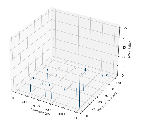
From above figure, it seems evident that at the beginning, i.e. when inventory left is high and time left is also high, the DQN agent is cautious while sending out the order. The order size (in lots) is smaller. But, as it gets close to end of time, the order size increases
Conclusion
With a deep dive hands on experience with Order Execution, we eventually found that RL definitely helps out in improved Order execution, better than some base cases. Further more, we can improve the execution algorithm by implementing more complication reward technique while utilizing LOB data.
Hope you enjoyed reading this exercise.
Appendix
References
- Optimal execution of portfolio transactions by Almgren, R. and Chriss, N. (2001)
- Reinforcement Learning for Optimized Trade Execution by Yuriy Nevmyvaka et al.