Portfolio Management using RL

Concerning Reinforcement Learning, Applications on 18 May 2021

Applications

In the earlier posts on RL, we talked about various algorithms, such as DQN, A3C, DDPG etc. But, how great it would be to apply these algorithms in the realm of Finance.

This post is dedicated to the very first Finance Use case of RL, viz, Portfolio Management. Without further ado, let’s deep dive into the problem statement and how we will frame the problem using RL.
So, sit back and grab your coffee.

Summary

As any RL problem, our goal is to maximize the reward. Here, the goal is to train multiple Deep Reinforcement Learning (DRL) agents to maximize Stock Portfolio performance over time.

Problem Description

An agent with a fixed capital $1,000,000 (\(C_0\)) wants to allocate the capital onto 2 (or more) stocks. Certain part of the capital (\(C_{reserve}\))is left aside for Cash reserve.

The agent should make buy/ sell/ hold decision everyday for each asset such that the portfolio value (composition of Cash reserve + present value of stocks) is maximized over time.

We will make this problem a continuous space - discrete action problem.

Data Requirements

High/ low/ Adjusted Close Prices for various stocks, downloaded from Yahoo Finance.

Mathematical Formulation

The portfolio consists of \(m\) assets + cash reserve. In our example, we will let \(m=2\).
The overall process can be formulated as a Markov Decision Process (MDP). In such MDPs, we need to construct a proper environment. We call this environment: PortfolioEnv.

The agent enters into the environment, and takes step, i.e. performs rebalancing activity in order to maximize the reward. Every step taken should take into account the below factors:

[1] Short Selling Not allowed
[2] Cash reserve should not become negative

Besides this, the environment also entails a Transaction Fee of 1 basis points, i.e. 0.01% of every notional traded.

Let’s define the more attributes pertaining to this environment.

1. Actions

   Since this is a discrete action space, we have defined the action space as below, with 7 unique actions.

        actions = [
            [-0.03, 0.03], [-0.02, 0.02], [-0.01, 0.01], 
            [0.0, 0.0], 
            [0.01, -0.01], [0.02, -0.02], [0.03, -0.03]]
   

   Let’s understand it in detail. Since, we are dealing with \(m=2\) assets, every action is of length 2. If \(v_t =\) $1M, we will sell $300K worth of asset A and purchase $300K worth of asset B under action [-0.03, 0.03].

2. State

   We will create 2 separate models for State (\(s_t\)) for the environment.

   • Vanilla State Memory (VSM):

     Each state \(s_t\) consists of the below features:

     • Return vector: For each stock, we will store the \(n\) recent daily returns. Vector length: \(mxn\)
     • Current Holdings: Latest portfolio holding of each asset (excluding Cash reserve). \(h_1, h_2 ...h_m\). The holding is normalized to initial holding of each asset. \(h_{1_t}/ h_{1_0}, h_{2_t}/ h_{2_0}\) Vector length: \(m\)
     • Cash reserve: Latest available cash \(c_t\). Normalized by initial cash
     • Permitted actions: Not all actions are feasible under a current state. What if the action taken leads to short selling? That action should be forbidden. For every action, it will be a boolean. 1 represents a permissible action, and 0 represents forbidden action. \(a_1, a_2.... a_{n_{actions}}\). Vector length: \(n_{actions}\)
       We have added the final item to make sure that agent learns NOT to take forbidden action

     
     Total length of state vector:
     \(m*n_{history} + m*1 + 1 + n_{actions}\)

     NOTE: This kind of state creation is inspired from Project work of Harish Kumar

   • Portfolio Vector Memory (PVM):

     This kind of state composition is inspired from the work done by Jiang, Xu and Liang.

     In this manner of state construction, we define the below state components:

     • Price Tensor: Asset price has 3 components – \(v_{high}, v_{low}, v_{close}\). We collect the price history of \(m=2\) assets for \(n_{history} = 30\) days.
       Shape of this tensor: \(m\) x \(n_{history}\)x \(3\)
       

     

     • Current Holdings: Current holdings weights in percentage terms. \(h_1, h_2 ...h_m\). Vector length: \(m\)
     • Cash reserve: Latest available cash (in percentage terms of overall portfolio ) \(c_t\).

3. Reward

   Constructing the reward is quite an art. The whole idea Reinforcement Learning is to maximize the cumulative reward. So, how we define the reward system in an environment is quite important.

   In the case of PortfolioEnv, immediate reward {r_t} has 3 key components:

   • Daily portolio return: This is how portfolio has gained or lost in a day.
   • Return variance Penalty: In order to avoid high volatile portfolios, we will grant a penalty based on portfolio variance
   • Forbidden action Penalty: If the agent takes a forbidden action, a significantyl high penalty is granted to that step.

   
   Hence, immediate action is given as below: \(r_t = \ln(p_t/p_{t-1}) - \beta_{variance} * var_p - \beta_{action} * bool_{forbidden}\)

4. Terminal State

   The agent will learn from the environment for a whole year. Terminal state is defined as the last day of the year.

5. Objective

   The agent’s obective is to maximize the discounted cumulative rewards:
   \(max \mathbb{E}[\sum_t \gamma^t.r_t]\), where \(\gamma: {discount factor}\)

Summarizing generic parameters used in creating the environment

Hyperparameter	Value	Description
Number of assets	2 (Ticker: APA, BMY)	Number of stock assets in portfolio
Initial Portfolio	USD 1M	Initial portfolio value
Initial cash	2%	Cash reserve at the beginning
Initial Holdings	Equi weighted	At the beginning, equal weight is assigned to each asset
Transaction fee	1 bps	Every buy/sell will hav a certain transaction cost
History	30 days	Number of historical records used in state vector
Variance Risk Penalize	0.08	Penalize factor to reduce portfolio variance
Forbidden Action Penalize	8	Penalize factor to avoid forbidden action
Discount factor	0.99	Discounts the future reward to today

Reinforcement Learning Agents and Network Topologies

We will use couple of RL algorithms (agents) utilizing both the worlds of Value based methods and Policy gradient methods

1. DQN with Vanilla State memory (DQN-VSM)

   For a detailed understanding of DQN, I would recommend the Deepmind paper in Nature. I will not go in the technicalities of DQN, but its application in this specific case.

   

   With state vector (VSM) as input, the output of the training model is the state action values pertaining to each possible action.

   Network Configuration as below:

   Hyperparameter	Value	Description
   mini batch size	32	number of training cases over which each Adam Optimizer is run
   replay memory buffer	200000	updates are sampled from this memory
   target network update frequency	50	The frequency (measured in number of episodes) to update the
   optimizer	Adam	Adam optimizer is used to train the network
   learning rate	0.0001	Optimizer learning rate
   clip value	100	Clips the final output of network to be between this -100 to 100
   initial exploration	1	initial value of \(\epsilon\) in \(\epsilon\) greedy exploration
   final exploration	0.1	final value of \(\epsilon\) in \(\epsilon\) greedy exploration
   final exploration frame	200000	number of frames over which \(\epsilon\) is linearly annealed to final value

2. A3C with Vanilla State memory (A3C-VSM)

   Refer to my previous article on A3C agent, and how it utilizes policy gradient technique to improve the policy. A3C incorporates 2 networks, viz, Actor and Critic.
   Actor defines the policy which the agent learns, i.e., probability of taking a particular action given the state.
   Critic criticizes the state value under the policy \(\pi\).

   The network models for both Actor and Critic are similar, with only difference is in the output.

   The asynchronicity comes from the fact that there are multiple worker agents trying to learn the policy while sharing the learnt network parameters regularly to the global Actor Critic model. A quick network A3C network recap:

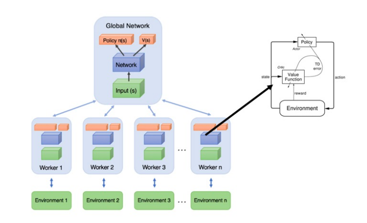
   Network Configurations (same for actor and critic) as below:

   Hyperparameter	Value	Description
   mini batch size	32	number of training cases over which each Adam Optimizer is run
   Number of cores	8 (and 1)	Number of cores on which the worker agents are trained. We will run both cases of multi core and single core.
   optimizer	Adam	Adam optimizer is used to train the network
   learning rate	0.0001	Optimizer learning rate

3. A3C with Portfolio Vector Memory (A3C-PVM)

   In this methodology, we will still utilize A3C agent, but the state definition comes from Portfolio Vector memory (as highlighted earlier).
   

   The network comprises of multiple CNN layers to utilize the effect of high/ low and close prices across past \(n\) days.
   NOTE: We have not used the forbidden action vector in PVM.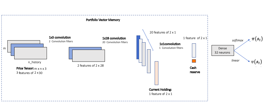

   

   Network Configurations (same for actor and critic) as below:

   Hyperparameter	Value	Description
   mini batch size	32	number of training cases over which each Adam Optimizer is run
   Number of cores	8	Number of cores on which the worker agents are trained
   optimizer	Adam	Adam optimizer is used to train the network
   learning rate	0.0001	Optimizer learning rate
   Network Layers	2 1x3 Convolutional Layers 20 1x28 Conv Layers 1 1x1 Conv Layer 32 neuron Dense Final Layer for Actor or Critic	PVM utilizes a large Deep Neural network.

Loss functions utilized in individual DQN and A3C agents are similar to the ones used in respective papers (DQN, A3C) published.

Let’s compare the performance of these individual learning agents.

Agent Performance Evaluations

The entire exercise is solely developed in Python (3.8+). For NN networks, keras has been used with tensorflow as backend.

As always, for detailed code and explanation, please write to me directly.

Without further ado, lets jump onto the agents and their learning patterns.

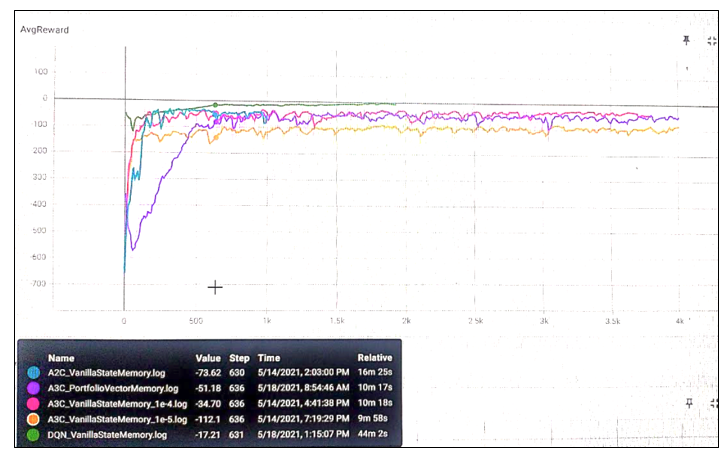
First of all, my apologies for such a bad resolution of the above result. My server machine is different and I cant take the screenshot directly. Camera resolution works only to some extent. So, what’s happening here?

There are 5 different agents learning to work their way around the environment

1. DQN-VSN:
   • Ran for 2000 episodes and training period was 1 year.
   • Started with lower rewards, but gradually agent started learning and cumulative reward started increasing.
   • Seems that even after 2000 episodes, cumulative reward was still going higher. This is a sign of over-fitting.
2. A3C-VSN with learning rate: 0.00001:
   • Worker agents running on 8 cores.
   • In total, ran for 4000 episodes and training period was 1 year. Each year was different for each worker.
   • Overall learning stopped quickly, i.e. maximum reward (for this agent) already achieved.
3. A3C-VSN with learning rate: 0.0001:
   • Similar functioning as above case, but a faster learning rate. (10x faster).
   • Agent slowly started learning, and maximum reward realized and saturated
4. A3C-PVM:
   • With a Deep CNN based Portfolio vector memory, this network and agent learns quite differently.
   • It started with quite a low reward, and started reaching new highs.
   • But, its learning is relatively slower than other networks.
   • 1 reason could be that this network doesn’t use the forbidden action vector.
   • However, eventually, the network learnt the best policy and achieved the best reward possible.
5. A2C-VSN :
   • Similar to other A3C VSM agents, but there is only 1 single worker.

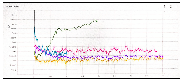
The below graphical summary compares the average portfolio value reached after \(n\) episodes for different agents. Clearly, DQN-VSM agent continues to learn (or over fits).

Agent Testing

• Our base case for the environment will be a Buy and Hold Strategy, i.e. we simply buy equi-weighted portfolio at the beginning of the period.
• Testing period: Year 2020. This year marks the most surprising and unprecedented year, both for financial markets and humankind in general. A period of Covid 19 took a lot of toll!
• Lets compare couple of strategies in this time frame.

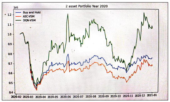
Seems like A3C-VSM model could have been a poor agent than just a Buy & Hold strategy for year 2020. However, DQN-VSM model has been shown an outstanding performance. Througout 2020, it kept on buying more of Asset 1 and selling asset 2. However, overall variance of DQN-VSM generated portfolio seems to be quite high.

Conclusion

This exercise was to get a hands on experience on Reinforcement Learning in Finance. I can guess that there would be few gaps here and there in the implementation and creation of states, actions, rewards etc.

I only considered a Continuous state space - discrete action space in this exercise. A more realistic and practical would be to consider a continuous action space as well. I would highly recommend you to create it from scratch. By doing a full hands-on, one can attain a deeper understanding of the topic.

---

Appendix

References

1. Deep reinforcement learning framework for the financial portfolio management problem by Jiang, Xu and Liang
   
2. Reinforcement Learning for Stock Portfolio Management by Harish Kumar
   
3. A3C Paper Asynchronous Methods for Deep Reinforcement Learning
   
4. DQN Paper Human-level control through deep reinforcement learning