[Momentum Investing] Part 3 - Risk Management and Portfolio Construction
In the last article, we analyzed risk and returns of prototype Momentum factors. There are a number of risks associated to investing in individual Momentum factors. For instance, these factors have negative skewness, i.e. they entail a heavy left tail risk.
In addition to the tail risk, Momentum can underperform during prolonged periods of range-bound price action, and signals used to identify Momentum can also become ineffective during such times.
On a single factor level, one can address the tail risk by introducing a ‘Stop loss’ overlay. The rationale behind a stop loss overlay is to prevent large losses during market turning points at the expense of a performance drag during false signals.
On a portfolio level, we can take advantage of cross-asset diversification. In this article we will further investigate how to combine single-asset Momentum Factors into an effective multi-asset portfolio. For instance, one needs to select a certain methodology such as Markowitz Mean Variance Optimization or Risk parity, and scale factors by asset volatility in a multi factor model. Diversification across asset classes cannot completely eliminate tail risk, but it can substantially dilute it as turning points do not occur in all markets simultaneously.
Risk Management
1. Stop Loss
Stop Loss is one of the most utilized risk management techniques among active investors and traders. Although stop-loss approach can be used both at the level of “individual assets” and “portfolio”, a more common approach is to overlay it at individual assets.
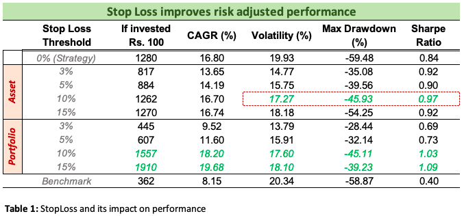
Figures 1 and 2 displays the Momentum portfolios’ performances when Stop Losses are applied at different levels. In fig 1, the SL is applied at individual asset level, which gets triggered whenever a particular asset falls below the specified StopLoss threshold. On the other hand, Fig 2 applies the StopLoss criteria at the portfolio level, i.e., whenever entire portfolio falls below a threshold of x%, all the assets are sold, and converted into Cash.
Table 1 displays the performance in both the case. As observed, the Stop Loss mechanism definitely lowers the risk, which can be observed both from reduced Volatility and reduced Drawdowns. Lower the stoploss trigger, lower the Volatility. However, that comes at the cost of lowering the upside as well. In both the scenarios, a trigger at 10% or 15% generated portfolios with higher Sharpe ratios. The portfolio level trigger worked even better, with a sharpe of over 1. This can be attributed to a consolidation risk that happens during the time of significant market downturs such as Covid 2020 event. Most of the assets individually breached the limits during the time. It may not have happened on the same day, and hence asset level portfolios underperformed. The portfolio level trigger, however, cut the losses on the entire portfolio by selling entire Equity stake until the next rebalancing date.
Another thing to note about the Stop Loss mechanism is when to apply the trigger. In our analysis, we are using daily Stop Loss triggers which are better to reduce the between-rebalance tail risks. Other approaches could be to apply such triggers at lower frequency such as weekly or during rebalancing dates only.
In summary, introduction to Stop Loss based Risk mechanism can modestly improve the Strategy’s risk adjusted performance.
2. Diversification Benefits
Asset Allocation Approaches
So far, in all our analysis, we had assumed a very basic asset allocation scheme, i.e. Equal Weighted portfolio - at every rebalance period, the chosen assets were assigned the same weight. But, is the same weight to all the assets good enough? In this section, we will explore other schemes of asset allocation, listed as below (ofcourse, this list is not at all exhaustive)
- Risk Parity Portfolio: The main aim is to find weights of assets that ensure an equal level of dollar risk,
- Mean variance Optimized Portfolio (MVO): developed by Harry Markowitz under Modern Portfolio theory, allows to generate a risk adjusted portfolio based on investor’s risk aversion
- Global Minimum Variance Portfolio (GMVP): delivers a portfolio that would have minimum variance at given point
- Max Sharpe Portfolio: as the name suggests, portfolio would observe high Sharpe at given point
- Max Returns Portfolio
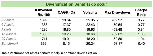
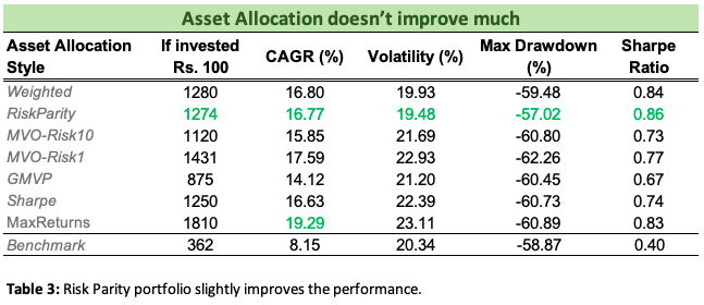
Figure 3 and Table 2 illustrates the portfolio’s historical performance under different asset allocation scheme. As one would have imagined GMVP to have lowest variance, but thats not the case. Reason is pretty straight forward. The weights are optimized based on historical performance. Similarly, the Max Sharpe portfolio doesnt have the maximum Sharpe for the same reason.
In all these schemes, only Risk Parity portfolio stands out, with higher Sharpe, contributed mainly by lower Volatility.
Introducing other factors
Momentum investing is not just about Price momentum, it can be any other factor related to company’s growth. Be it absolute revenue growth, or a more normalized Earnings Per Share growth. In this section, let’s see what happens when we incorporate the Earnings Momentum along with our price momentum factors.
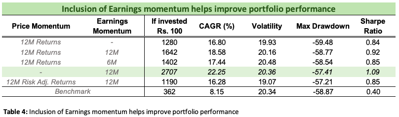
As illustrated in Figure 4, a pure 12-month trailing Earnings Momentum based model generated more alpha than our base prototype with just 12-month Price momentum. Trying out different combinations also illustrate the similar story, that Earnings momentum denifitely yield a better Momentum portfolio than a vanilla one.
Conclusion
Risk management is extremely crucial for any portfolio. Extreme portfolios are not everyone’s cup of tea, and with right risk mitigation techniques, one can avoid these extreme market behaviours. In this article, we highlighted few techniques about Risk management, such as Stop Loss, and how a simple Stop Loss helped reduce the portfolio volatility from 20% to nearly 17%. With lower volatility, these portfolios even showcased higher Sharpe, implying that investors didnt have to compromise too much on the absolute returns for the lower level of risk. Furthermore, asset diversification also helped reduce the volatility by over 100 bps, by introducing 15 assets, 5 more than our base prototype.
Towards the end, we introduced that a portfolio need not always be an Equi-weighted portfolio. In our analysis, a risk parity based asset allocation technique fared better than the Equi-weighted. Ofcourse, there is no shortage of more sophisticated approaches. A simple search on various platforms can provide various techniques.
Lastly, we presented the introducted of other factors, such as Earnings Momentum, and how its introduction can further help improve the performance.
Now, we are ready to combine all our studies together. In the next article, the last for this series, we will uncover incrementally enhanced portfolios which will incorporate learnings from different parts of this study. Till then, stay tuned!
Appendix
- Research Details & Source: Project Quant, by Ankit Gupta
PS: For detailed python notebook, you can reach out to me directly!
Disclaimer: The article is solely made available for educational purposes and doesn't promote any investment or trading guidance whatsoever. Any views or opinions presented in this article are solely those of the author.